Benchmarking ML-DSA Signature Generation: Understanding Rejection Sampling Performance
Introduction
As post-quantum cryptography (PQC) adoption accelerates, developers face new challenges in deploying signature schemes like ML-DSA on constrained devices-from embedded IoT devices to edge servers with limited computational resources. Unlike traditional signature algorithms such as RSA or ECDSA, which typically exhibit relatively predictable signing latency on a fixed platform, ML-DSA introduces an architectural feature rejection sampling that makes signing time inherently variable. This probabilistic mechanism ensures cryptographic security but creates variable signing latencies that can significantly impact system performance.
In this post, we’ll explore what rejection sampling means for ML-DSA benchmarking, share concrete performance metrics, and discuss best practices for measuring signing speed on constrained cryptographic modules.
This post extends section 4.1 of IETF draft Adapting Constrained Devices for Post-Quantum Cryptography.
Why ML-DSA Signing is Different
ML-DSA implements the Fiat-Shamir with Aborts construction, which uses rejection sampling as a core mechanism - a design choice rooted in lattice-based cryptography’s unique mathematical properties. Here’s what that means practically:
The Fiat-Shamir with Aborts Construction
Traditional Fiat-Shamir signatures use a public challenge derived from the message and public key. However, lattice-based signatures like ML-DSA need stronger guarantees. The “with Aborts” variant solves this by:
- Computing preliminary signature components (called a “y” value in lattice terms)
- Deriving a challenge from these components and the message
- Computing candidate signature components using the challenge and secret key
- Checking norm bounds: Verifying that these components don’t exceed predefined thresholds
- Either accepting the signature or aborting and restarting with fresh randomness
What the Norm Bounds Actually Do
The norm bound checks ensure that signature components stay within specific vector magnitude ranges. In lattice cryptography, if signature values are allowed to vary based on the secret key properties, an attacker could observe:
- Patterns in signature magnitudes that leak information about the private key
- Subtle correlations between multiple signatures that compromise security
- Bias in the distribution of valid signatures
By enforcing strict bounds, rejection sampling eliminates these side channels. The tradeoff: some attempts must be discarded, creating the variable latency we’ll see throughout this post.
Why This Creates Variable Performance
After computing candidate signature components, the algorithm checks whether these bounds are satisfied. If they aren’t met - which happens probabilistically - the entire signing attempt is discarded and restarted with fresh randomness.
This approach serves two critical purposes:
- Security: Prevents information leakage about the secret key through out-of-range values
- Correctness: Ensures signature distributions match security proof assumptions
Unlike traditional algorithms that process a message once and produce a signature, ML-DSA may need to retry the signing process multiple times. This makes predicting signing latency fundamentally different from RSA or ECDSA.
The Numbers: Rejection Probability and Expected Attempts
Here’s where benchmarking gets interesting. The acceptance probability - the chance a signing attempt succeeds on the first try - varies by ML-DSA parameter set:
| ML-DSA Variant | Acceptance Probability | Expected Attempts |
|---|---|---|
| ML-DSA-44 | 23.50% | 4.255 |
| ML-DSA-65 | 19.63% | 5.094 |
| ML-DSA-87 | 25.96% | 3.852 |
What this tells us:
- ML-DSA-44 (compact variant) succeeds about 1 in 4 times per attempt
- ML-DSA-65 (NIST Category 3, most deployed) expects roughly 5 attempts on average
- ML-DSA-87 (highest security) actually has the best acceptance probability, requiring ~3.9 attempts
These aren’t guesses - they’re mathematically derived from the algorithm’s structure and parameters defined in FIPS-204 using Equation 5 from Li32, assuming a random bit generator (RBG) as specified in Section 3.6.1.
Factors Affecting Rejection Probability
The probability that any given signing attempt succeeds isn’t fixed - it depends on several factors:
- The message being signed: Different messages produce different challenge values
- The secret key material: Specific key properties affect norm bound satisfaction probability
- Random seed (hedged signing): When FIPS-204 Section 3.4 hedged signing is used, additional randomness affects outcomes
- Context string: The optional context parameter (FIPS-204 Section 5.2) influences the challenge derivation
In practice, this means some message-key combinations may require significantly more rejection iterations than others. A particular message signed with a particular key might consistently need more attempts than average, while another pairing might consistently succeed quickly.
Understanding the Distribution
The expected number of attempts is only part of the story. Due to the geometric distribution of the rejection-sampling loop, we need to understand the “tail” of the distribution-what happens in worst-case scenarios.
The Mathematical Model
For benchmarking and capacity planning, the rejection-sampling loop is well modeled as a geometric distribution with acceptance probability \(p\):
- Each attempt either succeeds (with probability p = acceptance probability) or fails (with probability \(1-p\))
- The number of attempts follows a geometric distribution
- The expected total attempts = \(1/p\) (the reciprocal of acceptance probability)
Using this model, we can calculate the cumulative distribution function (CDF)-the probability of completing signing within exactly N iterations.
ML-DSA Cumulative Distribution
The CDF expresses the probability that the signing process completes within at most a given number of iterations.
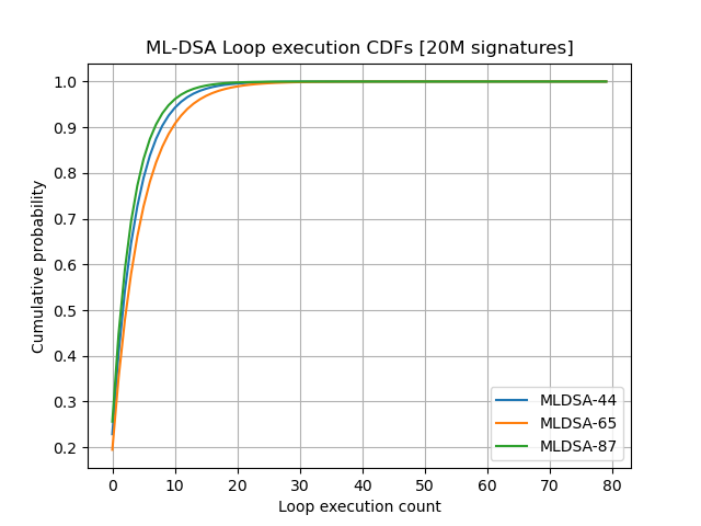
The data shows significant variation across ML-DSA variants:
- First attempt success: Only 19.6% to 26% of signing operations succeed on the first try
- Within 5 iterations: About two-thirds (67-78%) of operations complete by the 5th attempt
- Within 10 iterations: Most operations (88-95%) complete within 10 attempts
- Tail behavior: Even after 11 iterations, a small fraction (3-9%) of operations still need more attempts
| Iterations | ML-DSA-44 | ML-DSA-65 | ML-DSA-87 |
|---|---|---|---|
| 1 | 23.50% | 19.63% | 25.96% |
| 2 | 41.48% | 35.41% | 45.18% |
| 3 | 55.23% | 48.09% | 59.41% |
| 4 | 65.75% | 58.28% | 69.95% |
| 5 | 73.80% | 66.47% | 77.75% |
| 6 | 79.96% | 73.05% | 83.53% |
| 7 | 84.67% | 78.34% | 87.80% |
| 8 | 88.27% | 82.59% | 90.97% |
| 9 | 91.03% | 86.01% | 93.31% |
| 10 | 93.14% | 88.76% | 95.05% |
| 11 | 94.75% | 90.96% | 96.34% |
This demonstrates the importance of dimensioning systems with adequate retry budget. While ML-DSA-44 and ML-DSA-87 show faster convergence than ML-DSA-65, all variants exhibit the same geometric tail behavior-rare but real outliers that extend beyond typical case scenarios.
Practical Implications for Constrained Devices
For battery-powered IoT devices and embedded systems, this variability matters significantly:
Latency Unpredictability
Consider a concrete example: suppose a single rejection-sampling iteration takes 100 microseconds on your embedded device.
- Best case (1 iteration): 100 microseconds
- Expected case (5 iterations): 500 microseconds
- 95th percentile (11 iterations): 1,100 microseconds
- 99th percentile (21 iterations): 2,100 microseconds
For time-critical applications like IoT gateways expecting 1 millisecond response times, this becomes problematic. If your system budgets for average-case performance (500 μs) and occasionally encounters 99th percentile cases (2,100 μs), you’ll miss deadlines approximately 1% of the time. In production systems handling thousands of signatures per day, that 1% isn’t negligible.
Energy Consumption Variability
Power consumption scales directly with iteration count. On battery-powered devices:
- A “fast” signature (1 iteration) might consume 50 mJ
- The same signature might consume 250 mJ at expected case (5 iterations)
- Rare outliers (21 iterations) might consume 1,050 mJ
For devices relying on energy harvesting or with tight power budgets, this 20x variation between best and 99th percentile cases creates significant uncertainty. Devices must either:
- Over-provision battery capacity for worst-case scenarios
- Implement aggressive power limiting that reduces throughput
- Accept occasional failed signing operations when power budgets are exceeded
Impact on TLS Handshakes
In TLS 1.3 with ML-DSA, the server performs a signature during the handshake. On a mobile IoT device over cellular:
- Expected signing: ~500 μs (manageable within handshake timing)
- Occasional outliers: ~2,100 μs (visible latency increase; user-perceptible in some scenarios)
- Compounded with network latency and cryptographic verification, outlier cases can extend handshakes by 10-20+ milliseconds
For LTE IoT connections, this can push handshakes from 200ms to 220ms - noticeable but usually acceptable. However, on slower networks or with multiple signature operations, the impact multiplies.
System Design Considerations
- Real-time systems must allocate resources for 99th percentile (21 iterations), not average-case (5 iterations), unless they can tolerate occasional missed deadlines
- Energy-harvesting devices need to either buffer energy or implement adaptive signing strategies
- Communication protocols should not assume signing is faster than network operations
- Firmware updates and key generation (which don’t use rejection sampling) can be significantly faster than signing, creating performance asymmetry
Best Practices for Benchmarking ML-DSA Signing
If you’re benchmarking ML-DSA implementations on constrained devices, don’t fall into the trap of reporting a single timing number. Here’s what to measure:
1. Single-Iteration Signing Time
Measure the time for signature operations that complete in a single rejection-sampling iteration. This captures the best-case performance and shows the efficiency of the core algorithm without retry overhead. It isolates the fundamental speed of your cryptographic implementation and makes it comparable across different hardware platforms.
2. Average Signing Time
Report the average across a large number of signing operations using independent messages and randomness. Alternatively, report the time corresponding to the expected number of iterations (shown in the table above). This reflects real-world performance that users will actually experience, accounting for the natural variation in rejection attempts.
3. Iteration Reporting
The most important step: make the signing function report the actual number of rejection iterations used. This enables:
- Accurate averaging of multiple signing operations
- Correlation of timing/energy measurements with iteration count
- Identification of anomalies or implementation issues
Comparing to Traditional Signatures
To illustrate why rejection sampling benchmarking is different, consider RSA or ECDSA:
- Signing time is deterministic: You can measure a single 2048-bit RSA signature and get the same runtime within microseconds every time
- Energy consumption is predictable: An ECDSA-P256 signature consumes nearly identical energy regardless of message or key
- Performance metrics are straightforward: Report a single timing number; it accurately represents all signing operations
The choice of metric dramatically affects system design. Budget for average-case and 1% of your operations will timeout. Budget for 99% case and you’re over-provisioning resources by 4-5x.
Conclusion
The rejection sampling in ML-DSA’s signing operations is a carefully engineered security feature, not a limitation. It’s fundamental to how lattice-based signatures provide provable security against known attacks. But it does require a thoughtfully different approach to performance evaluation than you might expect from traditional signature algorithms. It is worth to note that:
- Performance is probabilistic, not deterministic. A single timing measurement is meaningless. Instead, you need to understand the distribution of signing times.
- The expected overhead is manageable. Averaging 4-5 iterations for ML-DSA-65 is reasonable. The core signing operation (one iteration) executes in acceptable time on modern embedded hardware.
- You can predict and measure it precisely. Using the geometric distribution model and FIPS-204 parameters, you now have the mathematical framework to estimate signing time distributions without extensive benchmarking.
- System design must account for variability. Real-time systems, battery-powered devices, and time-sensitive protocols need to budget for 99th percentile cases, not average-case performance.
- Signing only. The mechanism applies only to the signing operation. This abort/retry mechanism mechanism doesn’t apply to key generation and verification.